Preface

In my previous post, I developed a simple mean-reversion strategy based on an oscillating signal calculated from a stock’s distance to its 50-day simple moving average.

However, the results revealed a key shortcoming: the algorithm struggled to account for momentum, leading to poorly timed exits during parabolic moves—either too early or too late.

In this post, we’ll dive into momentum and conduct an analysis to validate our assumption. If we can confirm that incorporating momentum enhances the strategy, we’ll move forward with developing a more advanced approach to leverage it effectively.

Note : This article builds on the insights from the first post. If you haven’t read it yet, consider giving it a quick skim to catch up!

Hypothesis

In the previous strategy, we analyzed large periods of stock market history (1–2 years) to build probability statistics around a stock’s likelihood of mean-reversion. These probabilities informed our trading decisions. However, such broad timeframes encompass various market conditions—bull, bear, and flat phases—which the overall probability statistic fails to account for, instead averaging everything out.

Take TSLA as an example: it often experiences prolonged sideways consolidations that frequently precede exponential upward movements. By calculating probability statistics across many years, we overlook these distinct “states” of the stock, treating them as a single homogeneous dataset.

Key question: What if we could classify a stock into specific momentum states—such as ultra-bear, bear, flat, bull, and ultra-bull—and refine the previous strategy to incorporate these states?

Our hypothesis is that the data distribution differs significantly across these momentum states. Relying on aggregated statistics over a large period blends these distributions, leading to inaccurate conclusions and suboptimal trading decisions.

Method

This leads us to a straightforward plan of action:

1. Classify Momentum States: Identify the stock’s momentum states (e.g., ultra-bear, bear, flat, bull, ultra-bull) across defined window intervals.

2. Analyze Probability Distributions: Calculate probability statistics for each momentum state, treating them as distinct data distributions.

3. Incorporate Momentum into Strategy: When applying the strategy from the previous post, factor in the stock’s current momentum state and use its corresponding probability distribution to make trading decisions.

The goal is simple: validate our hypothesis that momentum states offer more precise insights, enhancing the strategy. And if the hypothesis doesn’t hold, we’ll still gain valuable insights.

Now, let’s crunch the numbers—grab your favourite drink and settle in!

Step 1: Defining the Momentum States

To start, let’s give each momentum state a clear, intuitive meaning:

1. ULTRA-BEAR: Severe downward movements leading to significant losses. Avoid holding positions during this time.

2. BEAR: Noticeable downward momentum causing losses. Consider avoiding positions or possibly going short.

3. FLAT: Sideways movement with minimal gains or losses. This phase is uneventful—better to allocate resources elsewhere or exploit consistent patterns here.

4. BULL: Upward momentum with notable positive returns. A good time to hold a position in the stock.

5. ULTRA-BULL: Intense market greed leading to parabolic upward movements. Ideal for holding positions, and perhaps leveraging with call options.

The challenge: We need mathematical definitions for these states. Let’s analyze TSLA to establish these definitions more broadly.

Return Distributions Over 3-Day Intervals

Our approach is straightforward: calculate stock returns over 3-day intervals and use those returns to classify momentum states.
While indicators like RSI or MACD could be used, actual returns better represent the “truth.”

IMO - Higher momentum should equate to higher profits, and vice versa.

I’m open to discussion on this point if you have alternative suggestions!

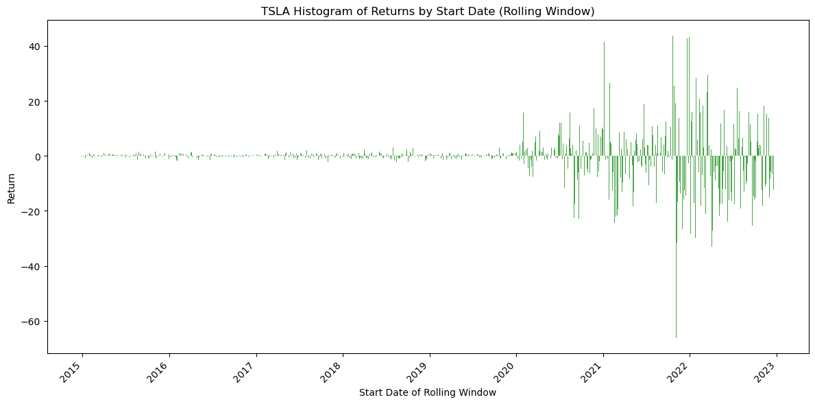
Absolute Distribution Over 15-Day Intervals

The chart below shows the dollar return for every point on the stock price, looking 3 days forward:

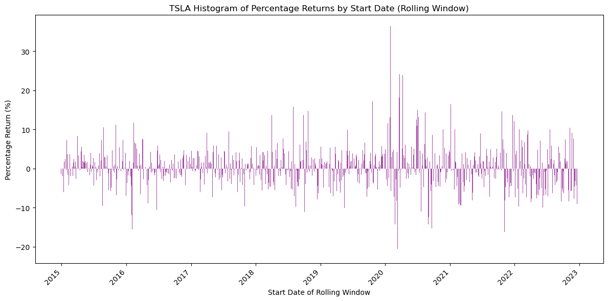
Percentage-Gain Distribution Over 3-Day Intervals

As noted in the previous post, absolute values introduce bias toward recent dates with higher stock prices. Instead, we analyze percentage gains for a more balanced view:

Determining Threshold Values

To divide the returns into five momentum states (ULTRA-BEAR to ULTRA-BULL), we calculate threshold values that evenly segment the data into five groups of ~500 days each:

thresholds = np.percentile(percentage_returns, np.linspace(0, 100, num_states + 1))

The resulting thresholds:

- [-21.29815971, -3.22985358, -0.61682303, 1.2045505, 3.61522128, 36.35119642]

Visualizing the Momentum States

The price chart below illustrates these momentum states, based on our thresholds:

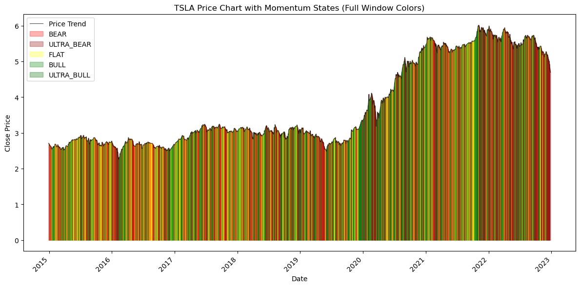
At this stage, we have a solid mathematical definition for each momentum state. The segmentation aligns well with intuitive patterns in TSLA’s price action, and we can move forward

Step 2: Probability Statistics for Each State

Now that we have identified 5 distinct momentum states:

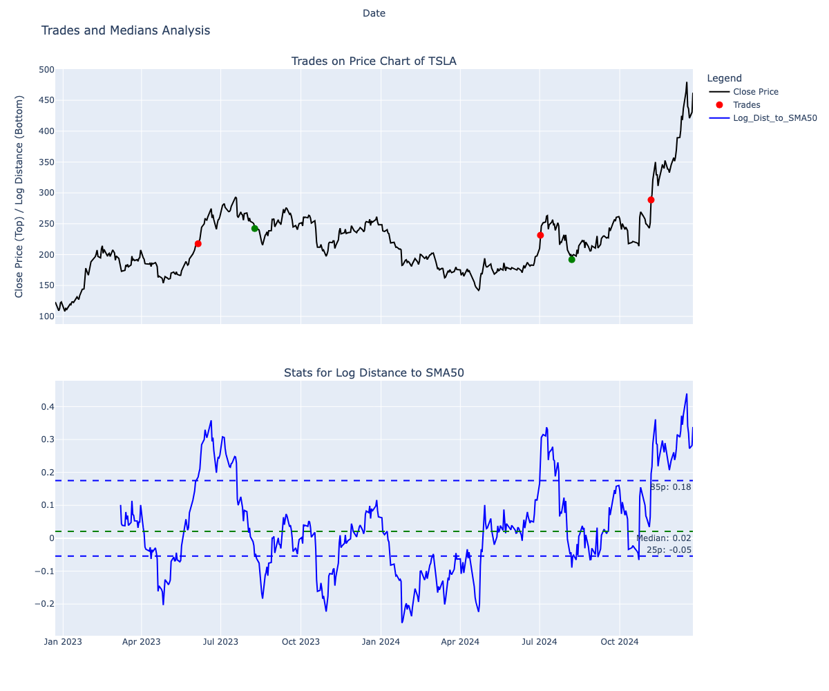
Let’s validate our assumption that these states represent separate data distributions by analyzing the Log Distance to SMA 50, as we did earlier.

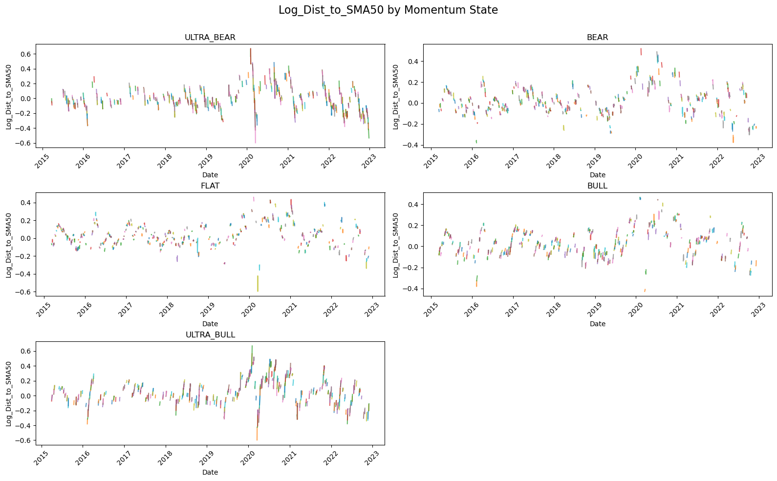
Visualizing Data Distributions

Instead of examining raw log prices, we visualize the data distributions as histograms for clarity:

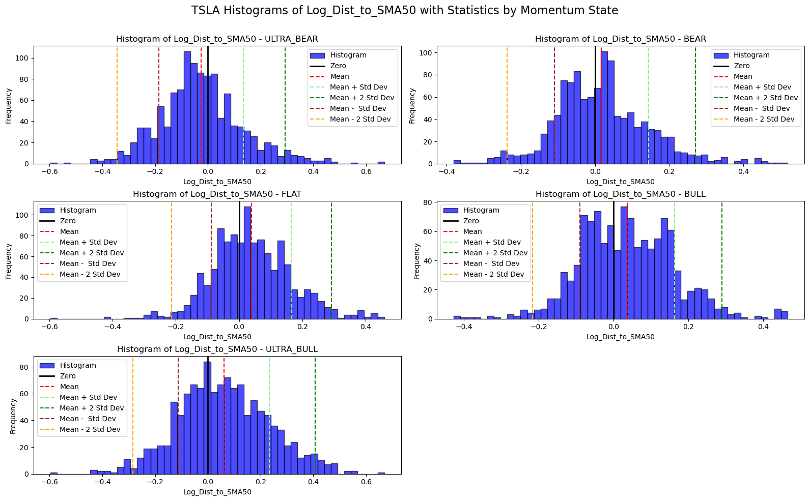
Key Observations

1. **ULTRA-BEAR** Skewed to the left, indicating most values are negative and below the SMA50.

2. BEAR: Symmetrical but slightly shifted to the left, with a narrower spread compared to other states.

3. FLAT:Nearly symmetrical and centered around zero, reflecting minimal deviation from the SMA50.

4. BULL: Symmetrical but slightly shifted to the right, with a narrower spread.
   5. ULTRA-BULL: Skewed to the right, indicating most values are positive and above the SMA50.

Summary

The data confirms that all momentum states exhibit distinct probability distributions.
These differences validate the need to consider separate statistics for each state when analyzing or trading.

Step 3: Simulating/Backtesting Based on Momentum States

Now that we have momentum-state definitions, let’s use this information to simulate trades.

Challenge: Estimating the Current Momentum State

To estimate the current momentum state, I use a simple heuristic for now (more in next blog):

1. Look at the past 3 dates, [t-6, t-5, t-4], and calculate the percentage returns and corresponding momentum states for those points.

2. Pick the majority (highest frequency) momentum state.

3. In case of a tie, randomly select one to avoid bias.
   Once the estimated momentum state is determined, I use only the probability statistics for that specific state. This allows the algorithm to contextualize current price movements based on similar past price structures, improving decision-making.

Simulation Using Momentum States

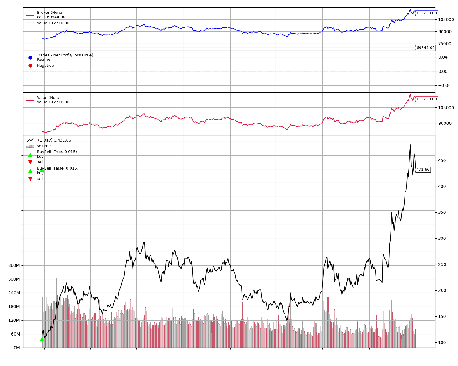
Baseline: Simple BUY-and-HOLD Strategy

First, let’s consider a baseline where we buy and never sell:

Our Momentum-Based Strategy

Next, we run the simulation using the momentum-state approach:

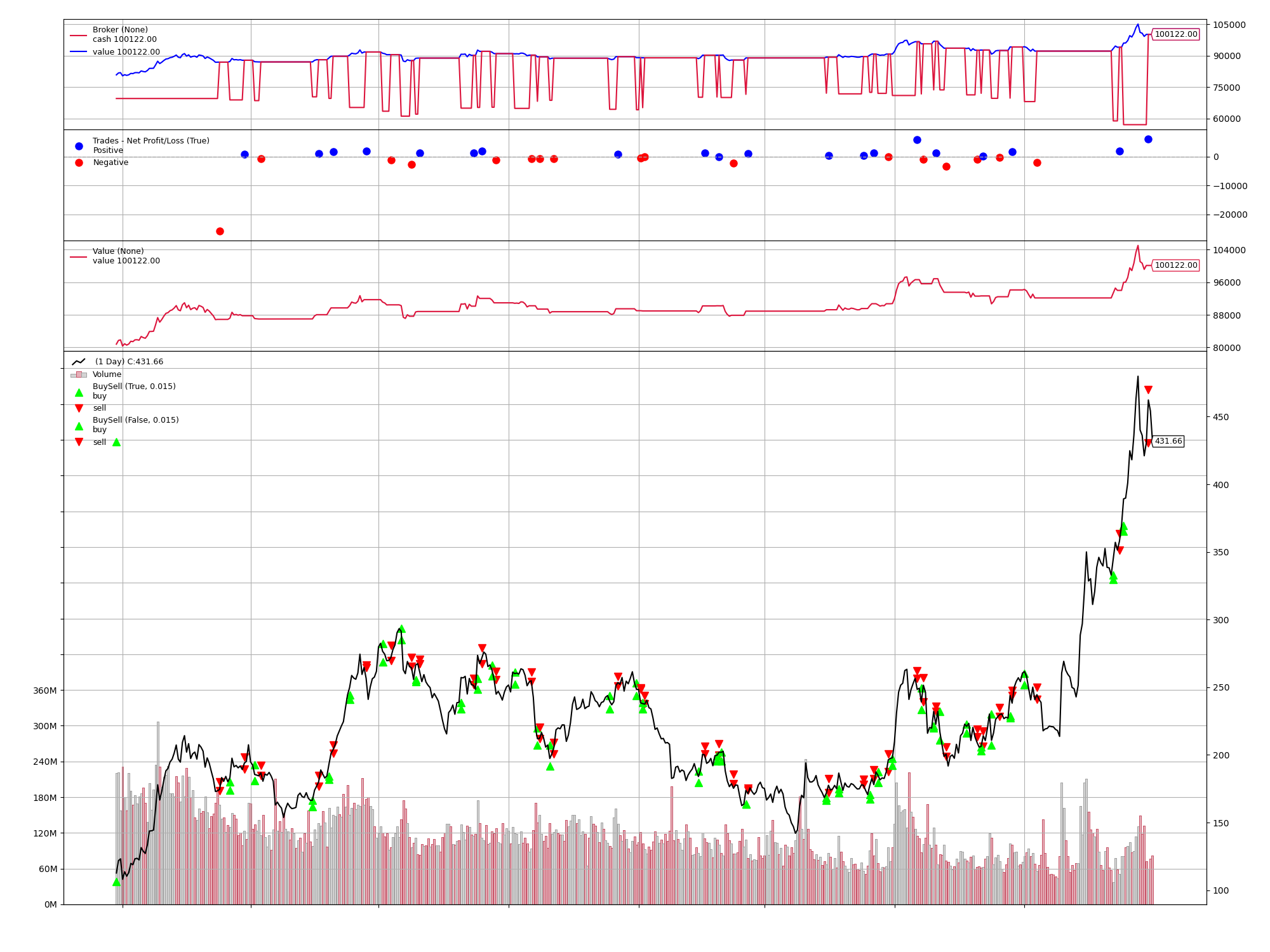
Side-by-Side Comparison

Comparing the two strategies:

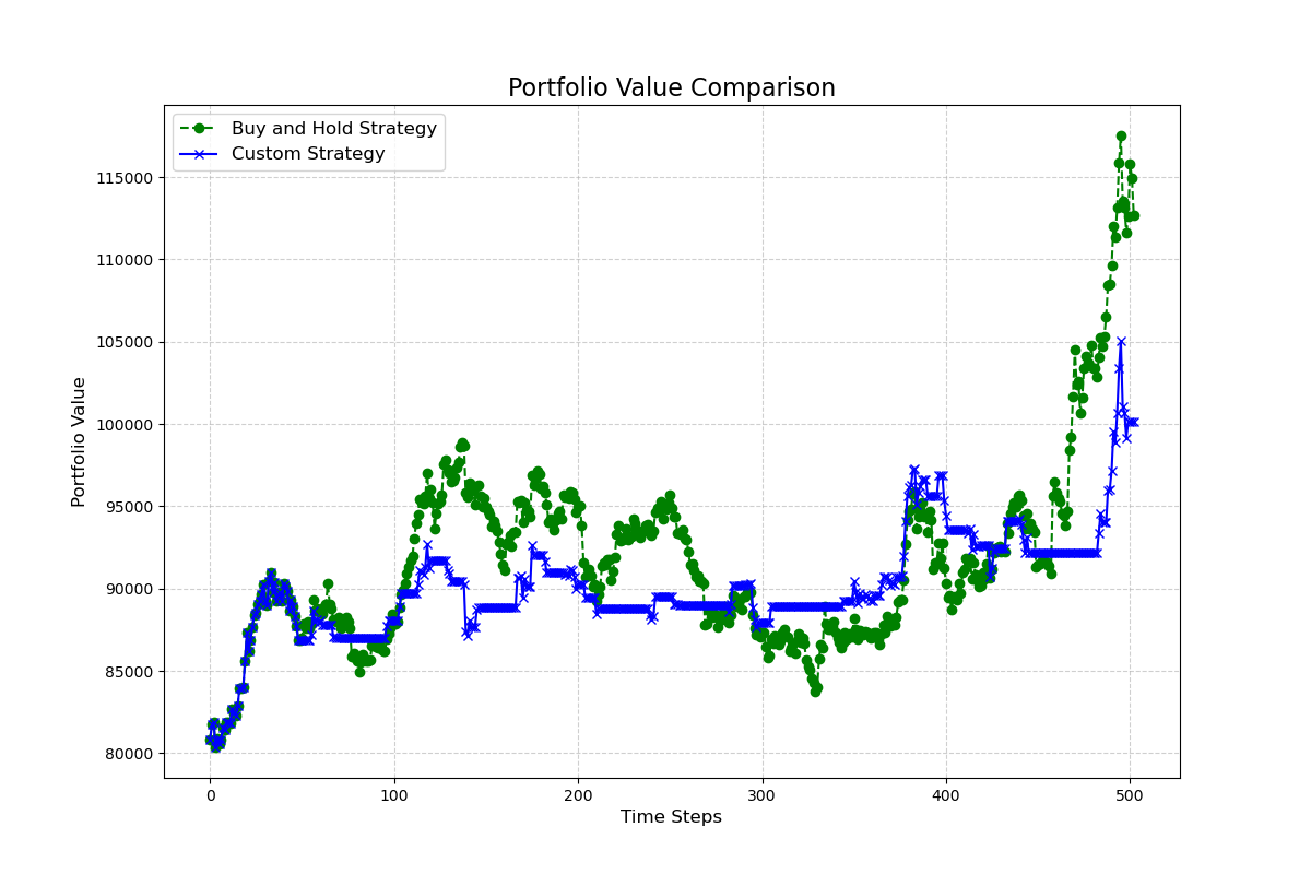
Observations

While the momentum-based strategy didn’t outperform BUY-and-HOLD overall, it demonstrated interesting results:

1. During significant price surges, the algorithm adapted and avoided blindly selling.

2. It showed agility by correcting itself, entering buy/sell positions after observing strong directional surges.

Examples of Strategy Adjustments

Changed to BUY after detecting a price surge: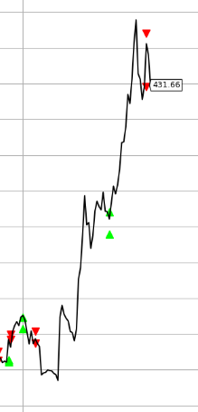

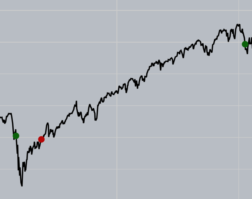
Avoided a big crash by adapting to the price structure: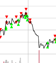

Compare this with trades from the previous strategy (without momentum consideration):

The older strategy exited parabolic moves prematurely because the statistics didn’t align with the observed price structure.

Conclusion

Although the momentum-based strategy didn’t beat the traditional BUY-and-HOLD, it showed clear improvements in agility and adaptability:

Agility: The algorithm adjusted to price surges and crashes dynamically.

Improved Contextualization: Considering momentum alongside oscillating signals enabled better alignment with price structures.

In the next post, I’ll explore building an ML model to predict the current momentum state, aiming to further enhance the algorithm. Stay tuned!