
Preface
I’ve been actively trading the markets for about 6 years now. Here’s an year-by-year retrospective of my trading portfolio (excluding my long-term investments which perform inline with indexes).
- Year 1 (2019) [Beginners Luck]: Got lucky with covid bull market. Felt like a god. Started learning technical-analysis, options and crypto.
- Year 2 (2020) [Massive loss]: Was humbled by the market. Realised I have much to learn.
- Year 3 (2021) [Learning]: Became much better at technical-analysis and options. Traded small, with an intention to learn. Bull market - Did well.
(I can only pull data from 2022 on my broker)
- Year 4 (2022) (-25%) [Learning]: SPY(-22%) Bear market, kept trades small to learn, made some good trades and some bad.
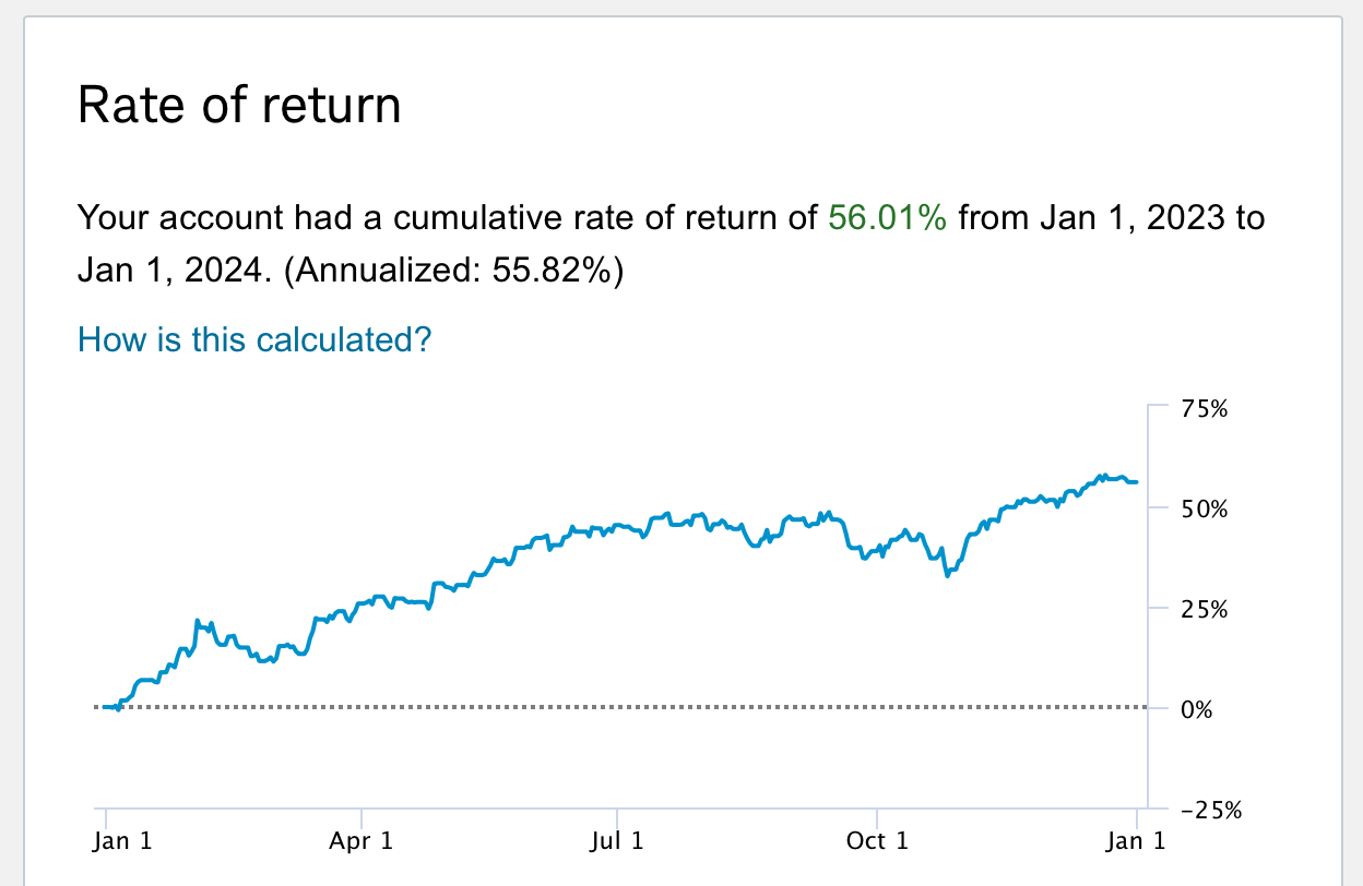
- Year 5 (2023) (+56%) [Outperform]: SPY (+24%): Screenshots below
- Year 6 (2024) (+52%) [Outperform]: SPY (+23%) - I actually did even better this year. Since I bought a house - I took a defensive stance, kept much higher cash positions and traded less.
- Year 7 (Jan25- May25) (+16.15%) [Outperform]: SPY (+1.39%) - Markets have crashed this year due to trump tariffs, were down 20% a few weeks back.
In summary: It took me years to learn. But it’s starting to bear fruit.
What strategy have I learnt?
I have 3 parts to my current strategy, and its quite simple.
- Discipline: For Investing - I plan for 5 years ahead. I allocate based on the plan, and I stick to the plan. This prevents me from making rash/too-risky decisions.
- Calculation: For Trading - Technical and Probabilistic Analysis are the backbone of my trading. To guide direction, size and timing of the trades - I use both TA and Probabilistic models. (Detailed in this post)
- Risk: I follow Nassim Talebs barbell-strategy. Most trades are on good quality companies - if I make a mistake, I feel comfortable holding long. I do take significant risky-trades with favourable risk-reward at times, but always in proportion.
How these posts are structured:-
- PART 1 & 2 - I explain my current probabilistic model. I use this as input information to my discretionary trades. I also backtest to show why my current options strategy works.
- Part 2.5: In Syncing via IBKR - I show how I collect historical data from broker with python.
- PART 3 - I build an ML Autoencoder + N-Gram predictive model that improves on the simple probabilistic model here. I show backtests on how this improves overall performance. (Yet to write this)
- PART 4 - I show how to automate this model with IBKR. (Yet to write this)
- PART 5, & Beyond - This is where I’m currently at. Exploring more complex ML & RL techniques to improve my strategy further.
My goal: is to inform and automate my trading strategy - so I can focus on my tinkerings with AI.
Who should read this post:
If you’re curious how statistics make money - hopefully I scratch that mental itch for you in this post series. There’s numbers, code, and insights - If that sounds interesting, I suggest you get your favourite drink at this point.
Let’s get started with an explanation of my simple probabilistic model.
Strategy 1 - Distance from moving average
Hypothesis
While stock prices generally move up and to the right, they typically oscillate around a moving average.
The 50 day moving average, is perhaps the most ubiquitous signal that traders take note of when making investment decisions.
We have 3 numbers here of note.
The stock price
The 50 SMA price
The difference between 1) and 2)
While the price and SMA are not oscillating number, their difference - the distance of the stocks price to its 50 day moving average is an oscillating number we can observe
Key insight What if we statistically identify when the stock is at the extremes - i.e too far above the MA, or too far below the MA from normal. Those could be good entry / exit points on the stock.
For the rest of the article, we will focus on number-3, the difference of price to its 50 day simple moving average (SMA)
Oscillations from mean
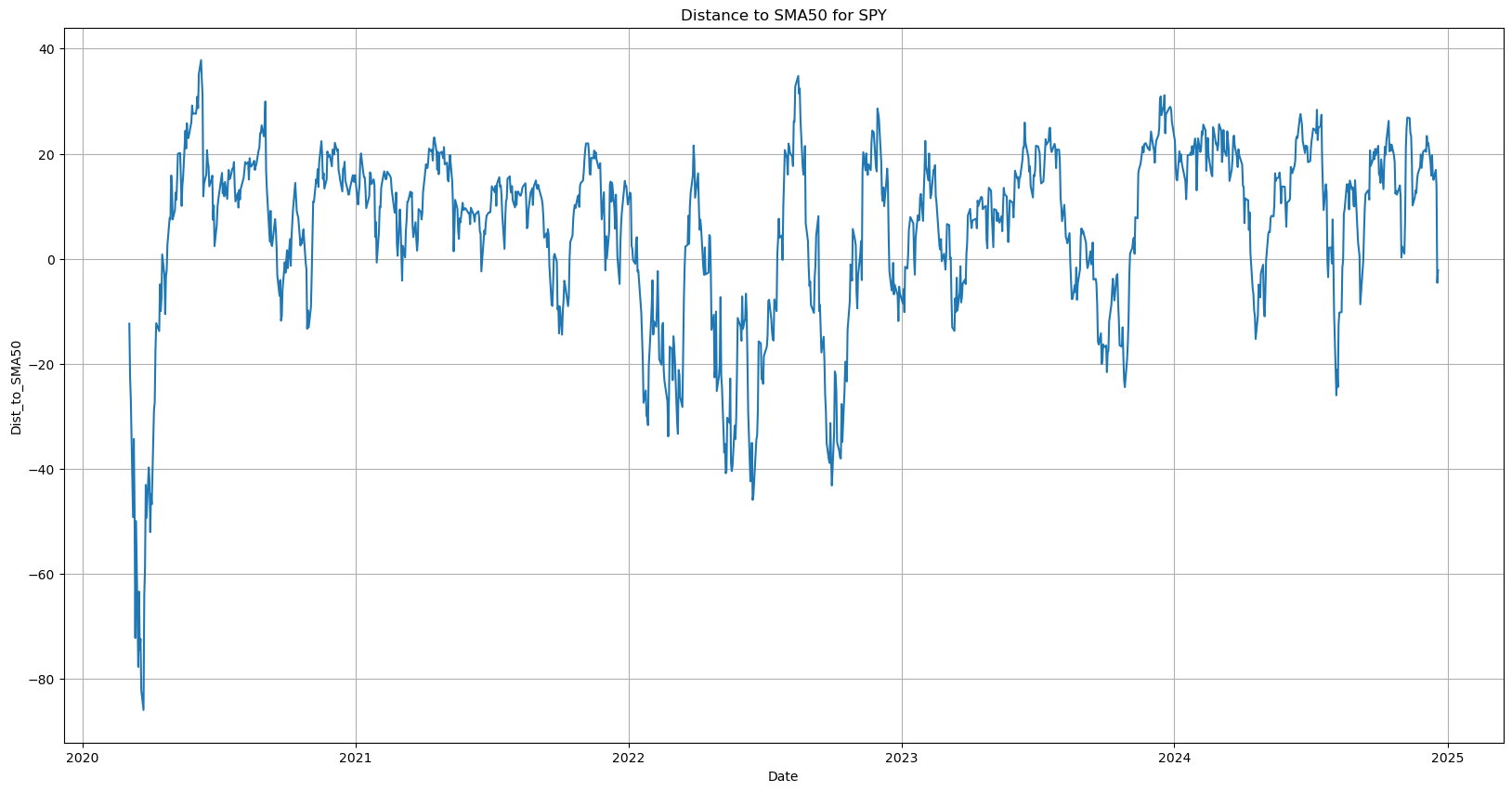
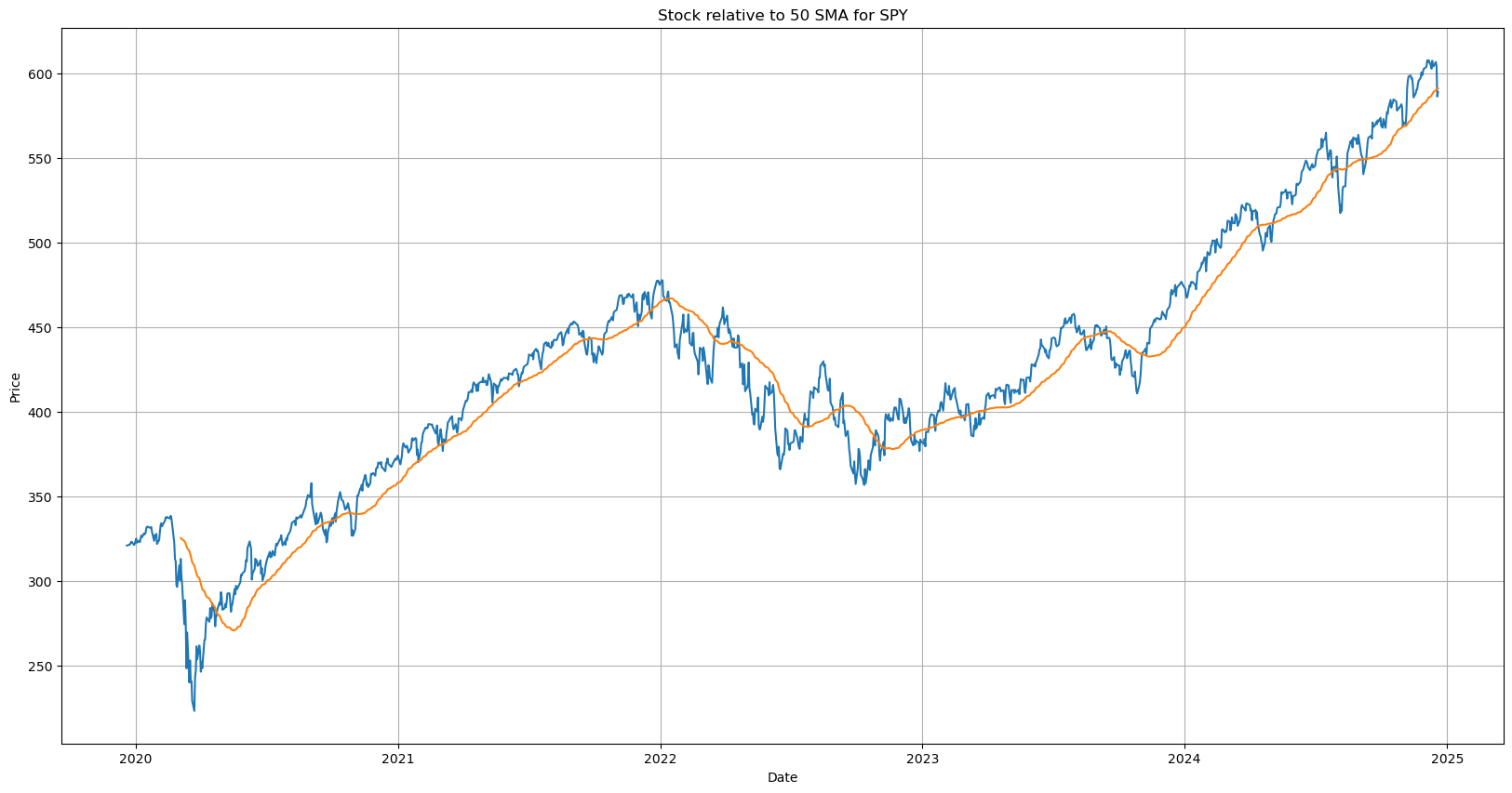
Plotting the Distance from SMA 50 for SPY gives us the above chart.
We’ve successfully found an oscillating pattern in the price structure.
Intuitively, its easy to visualise an average line and see the number oscillating above and below.
Let’s get more formal , and define some simple statistics of this number , namely - its average, median, standard deviation, and some percentiles.
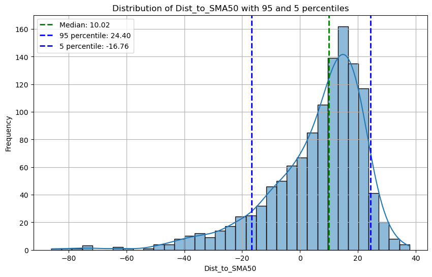
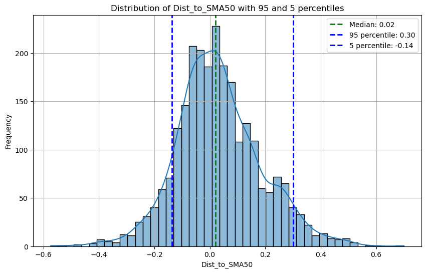
Distributions
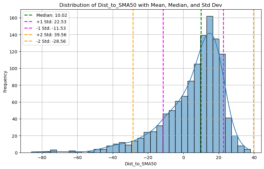
When we plot the frequency distribution of this number as a histogram, its easy to see that it fits a right-skewed distribution with its mean away and to the right of 0.
Note that the distribution is skewed towards the positive ( bull markets in the last 5 years ) , but its easy to see the sigmas.
I’m interested in the 95/15th percentiles - namely the 95 and 15 percentiles, let’s plot those too
Strategy insight
When the stock is more than $24.4 above its 50 SMA - There is a 95% chance it will go back to its median price soon.
Conversely, when the stock is more than $16.76 below its 50 SMA - There is a 85% chance that it will go back near its median price soon.
Caveats:
It’s also possible that the stock price itself keeps going down or remains stable, and the Moving average comes closer to the price to reduce the gap
The price will eventually come closer to the SMA, but we don’t know when. Stocks can remain irrational much longer than we can be solvent.
Nevertheless, the caveats may or may not happen - Let’s find out what actually happens.
Simulating the strategy
Instead of visualising this oscillating number, let’s plot these extremes on the stock chart itself
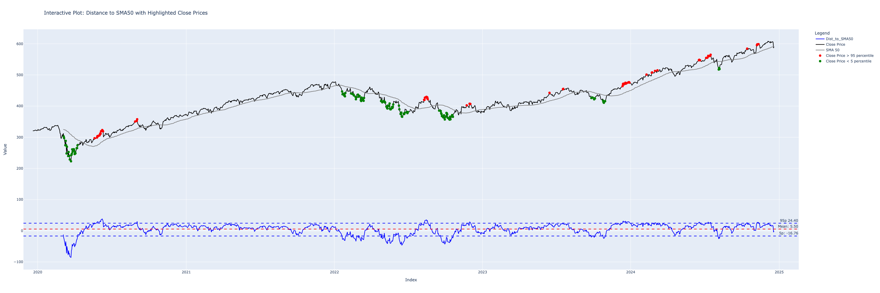
The lower indicator, shows the percentiles and mean overlayed on the oscillating chart. While the chart above highlights these extremes on the price chart itself.
Looks pretty good mostly - reds are sells, greens are buys. Problem solved? - Not really.
Let’s run the simulation, on what happens if we use this strategy. We buy on the green, if we have no stock - and sell on the reds if we have stock already with a simple simulation
def simulate_trades(data, highlight_low_indices, highlight_indices):
    # Initialize variables
    trades = []
    shares_owned = 100
    total_profit = 0
    buy_price = data['Close'][0] # Assuming starting prices

    # Simulate trades over the period
    for i in data.index:
        if i in highlight_low_indices and shares_owned == 0:
            # Buy action
            buy_price = data['Close'][i]
            shares_owned = 100
            trades.append({'Date': i, 'Action': 'Buy', 'Price': buy_price, 'Shares': shares_owned, 'Profit': None})
            print(f"Bought 100 shares at: {buy_price:.2f} on {i}")

        elif i in highlight_indices and shares_owned > 0:
            # Sell action
            sell_price = data['Close'][i]
            profit = (sell_price - buy_price) * shares_owned
            total_profit += profit
            trades.append({'Date': i, 'Action': 'Sell', 'Price': sell_price, 'Shares': shares_owned, 'Profit': profit})
            print(f"Sold 100 shares at: {sell_price:.2f} on {i}")
            print(f"Profit/Loss for this trade: {profit:.2f}")
            shares_owned = 0

    # Sell remaining shares at the last available price
    if shares_owned > 0:
        sell_price = data['Close'].iloc[-1]
        profit = (sell_price - buy_price) * shares_owned
        total_profit += profit
        trades.append({'Date': data.index[-1], 'Action': 'Sell', 'Price': sell_price, 'Shares': shares_owned})
        print(f"Sold remaining shares at: {sell_price:.2f} on {data.index[-1]}")
        print(f"Profit for this trade: {profit:.2f}")

    return total_profit, trades
Which gives us :-
Bought 100 shares at: 302.4599914550781 on 2020-03-05 00:00:00
Sold 100 shares at: 296.92999267578125 on 2020-05-20 00:00:00
Profit for this trade: -552.9998779296875
Bought 100 shares at: 446.75 on 2022-01-20 00:00:00
Sold 100 shares at: 419.989990234375 on 2022-08-10 00:00:00
Profit for this trade: -2676.0009765625
Bought 100 shares at: 385.55999755859375 on 2022-09-16 00:00:00
Sold 100 shares at: 402.4200134277344 on 2022-11-23 00:00:00
Profit for this trade: 1686.0015869140625
Bought 100 shares at: 425.8800048828125 on 2023-09-26 00:00:00
Sold 100 shares at: 464.1000061035156 on 2023-12-12 00:00:00
Profit for this trade: 3822.0001220703125
Bought 100 shares at: 517.3800048828125 on 2024-08-05 00:00:00
Sold 100 shares at: 584.3200073242188 on 2024-10-14 00:00:00
Profit for this trade: 6694.000244140625

Total Profit over 5 years: 8973.001098632812
Pretty good! We made $8,973!!
Naah, you’d do better just to buy and hold the shares. If you just held , your profit was - $27,014.99
So in affect, this strategy is actually pretty bad: -$18,041.99 bad. Woops.
What went wrong ?
Problem 1 - Momentum
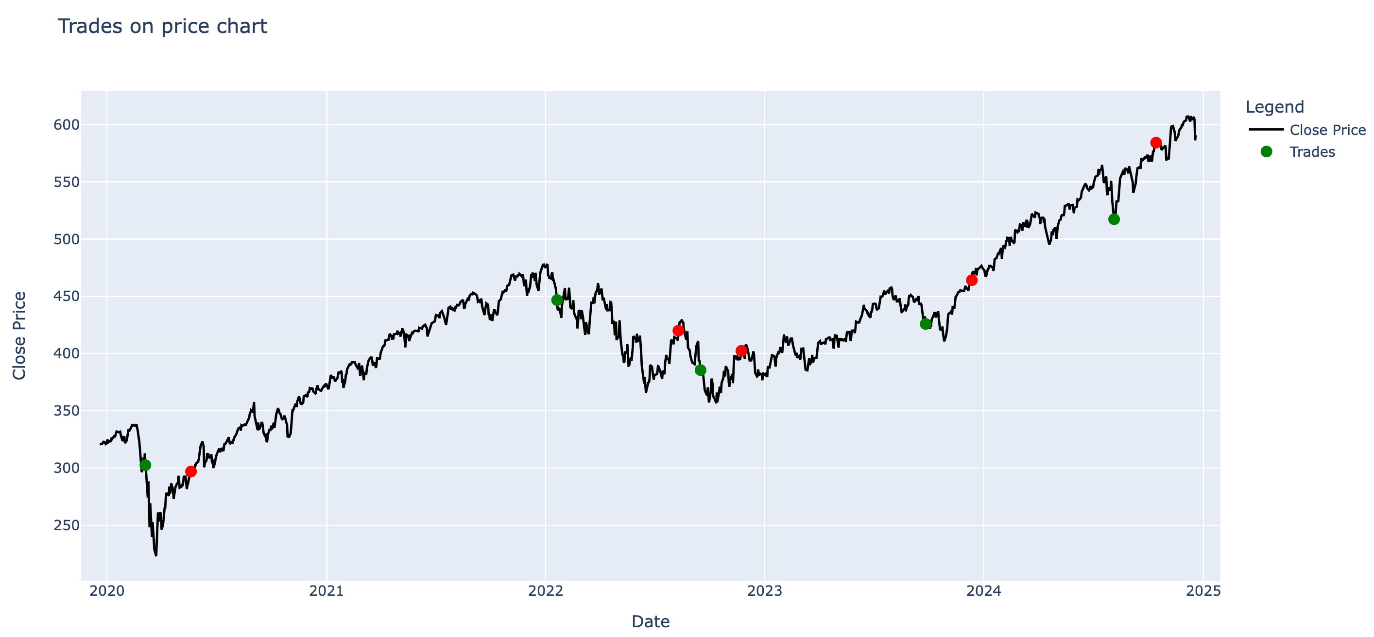
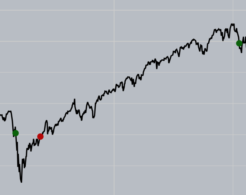
If we plot the trades on the chart - the problem is clear. The red markers are failed trades. Notice that after the red markers - the stock continues to climb much farther and they typically are in bull runs.
At times, the strategy works - but other times, especially in periods of high momentum - low stock prices go lower, and high stock prices go even higher. These period of high momentum, make us exit the strategy too soon and we lose out on massive gains.
Problem 2 - Bias
There is an obvious problem with our solution. We are calculating the statistics on absolute numbers with 10/10 hindsight bias.
Since we already know the prices historically, ofcourse the math will line up. But future price movements can be quite different from the past.
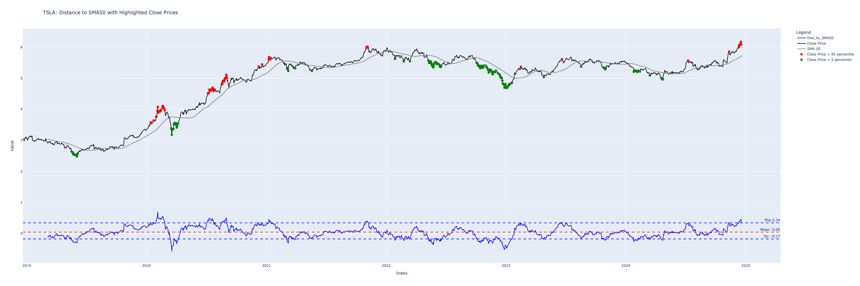
SPY is a very stable stock, and so this problem is not so obvious - let’s plot the extremes on TSLA chart instead, to show how a much more volatile stock behaves
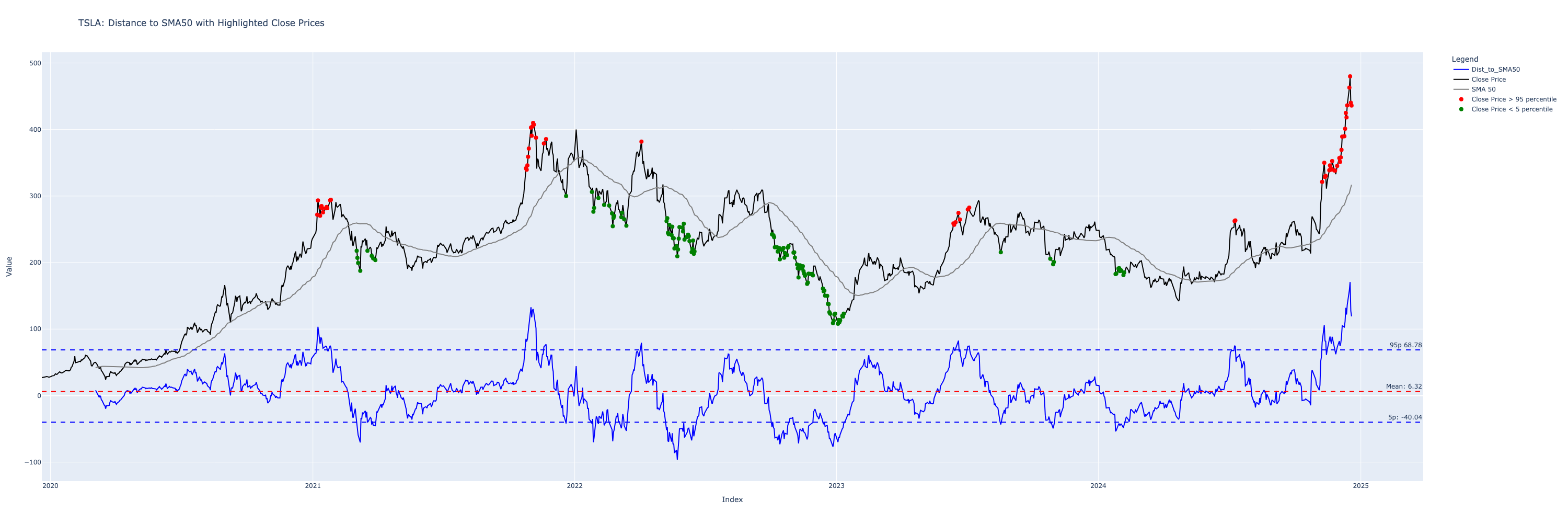
Notice what happens at the end, when TSLA stock recently went parabolic, every points on the chart are showing as SELL!
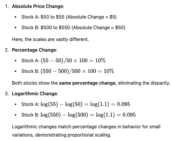
In absolute terms -
10% gain on a $500 stock = $50
10% gain on a $50 stock = $1
those numbers are a factor of 50 apart! for the same percentage gain.
Another way to see this bias is by plotting a longer timeframe on the oscillating distance chart
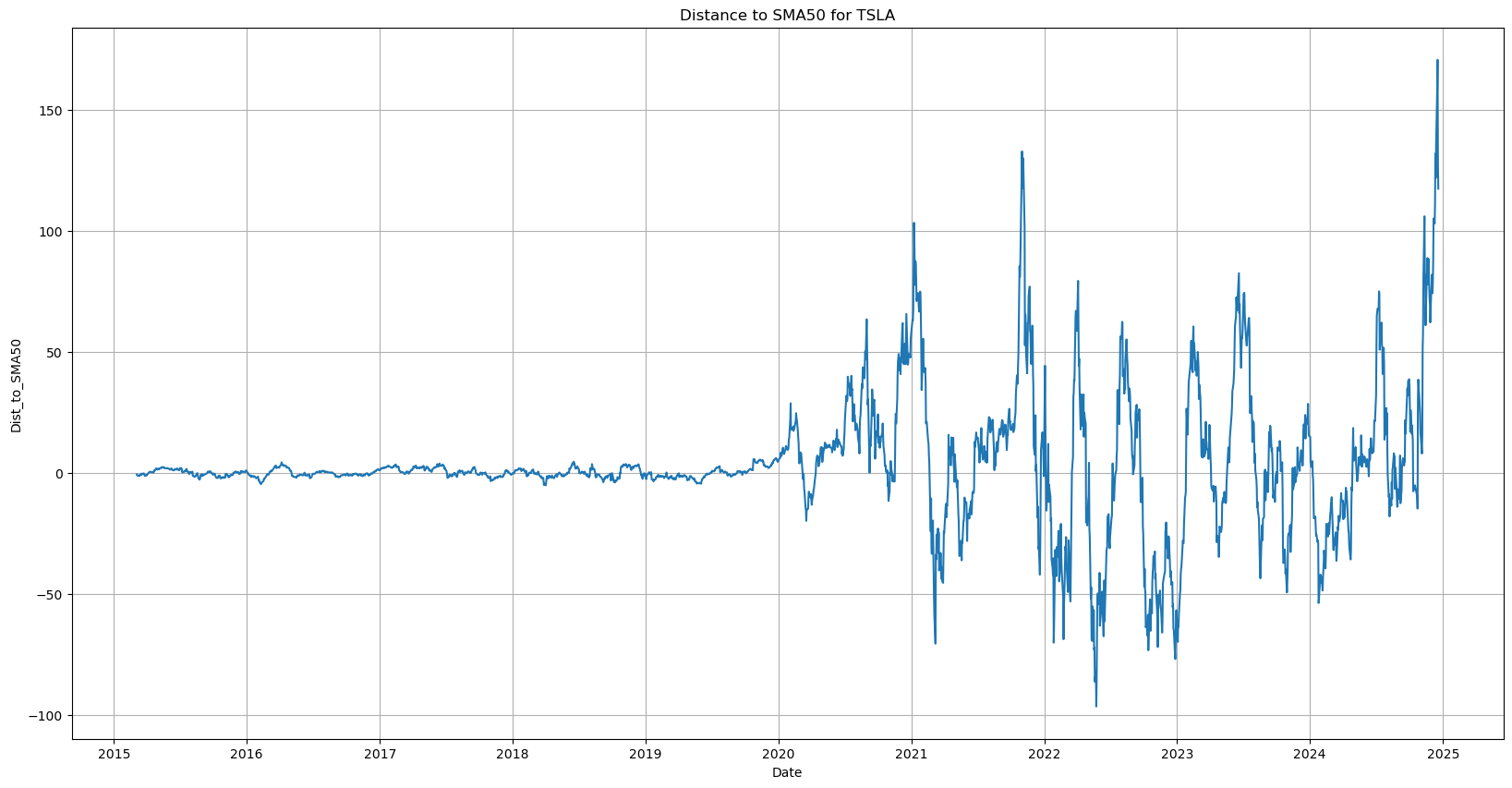
When the stock price was in absolute terms low, the variation on the distance converges to 0 on the left.
Let’s fix the issues
Fixing the bias
We could simply compare the %age movement, instead of the absolute values to fix this bias.
But, what if we can do a simple transformation that can be more broadly applicable to all the strategies in the future and remove this problem altogether?
Log is an simple solution here -
When we compare Log(price), the differences have the same relative magnitude and remove this problem.
To demonstrate:-
It’s also a simple one line fix - we Log the close prices right after fetching them in the beginning. (but we’ll keep separate columns to make things maintainable)
data["Close"] = np.log(data["Close"])
Now the Long-term chart has more uniform oscillations
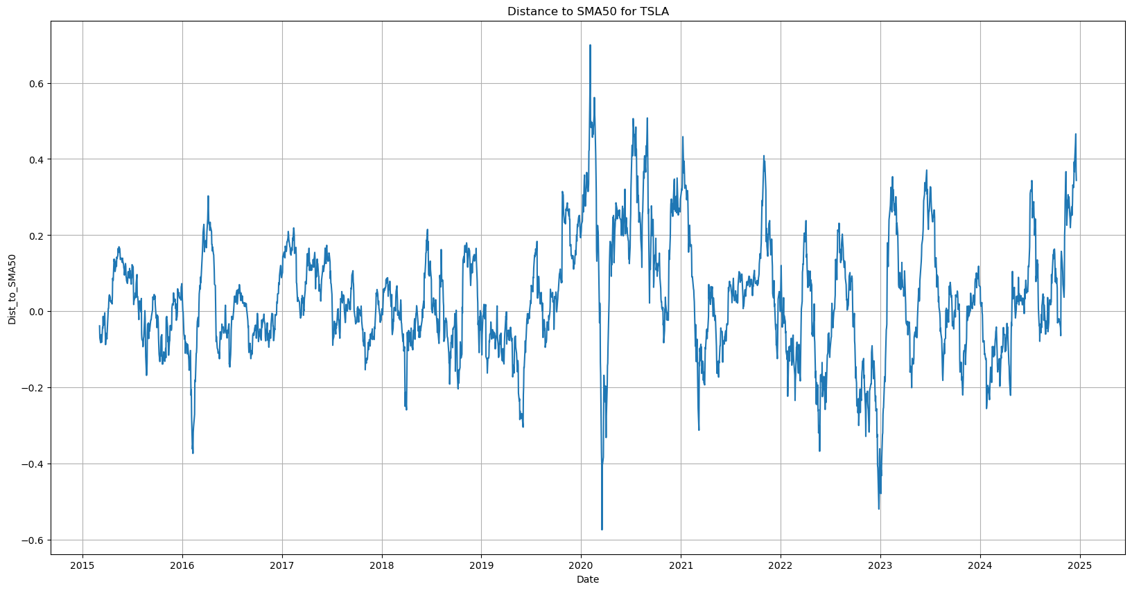
And our distributions are also less skewed
Plotting extremes on Log prices
Just for comparison, this was the before image (note the y scales are different, so its not an exact comparison)
Also - we should split the data in train, test and validation - because we don’t want to have the hindsight bias, and this reflects actual conditions much bette.r
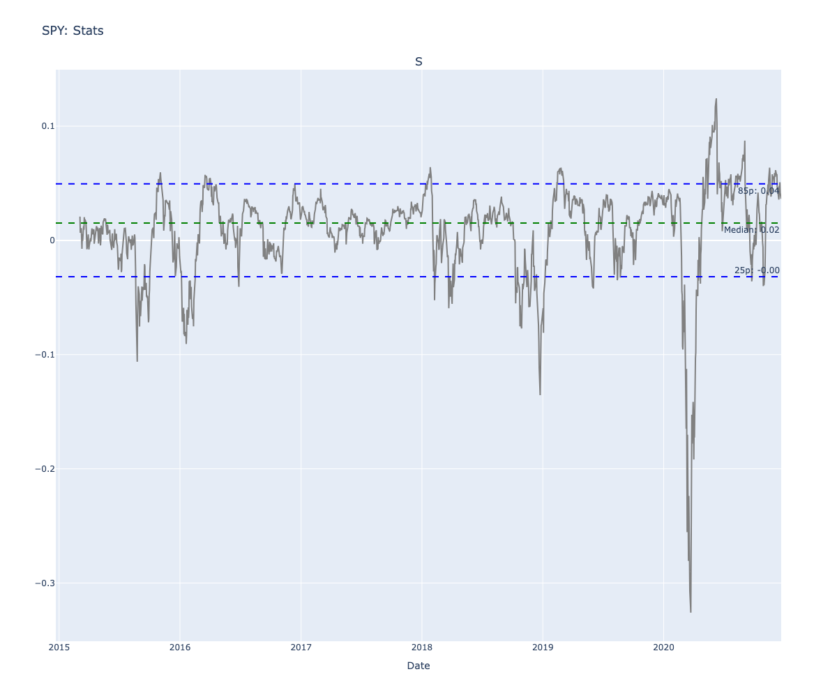
Let’s run the statistics for SPY again, before we run the simulation again.
Statistics for Log Distances:
Highlighting extreme points on test price chart
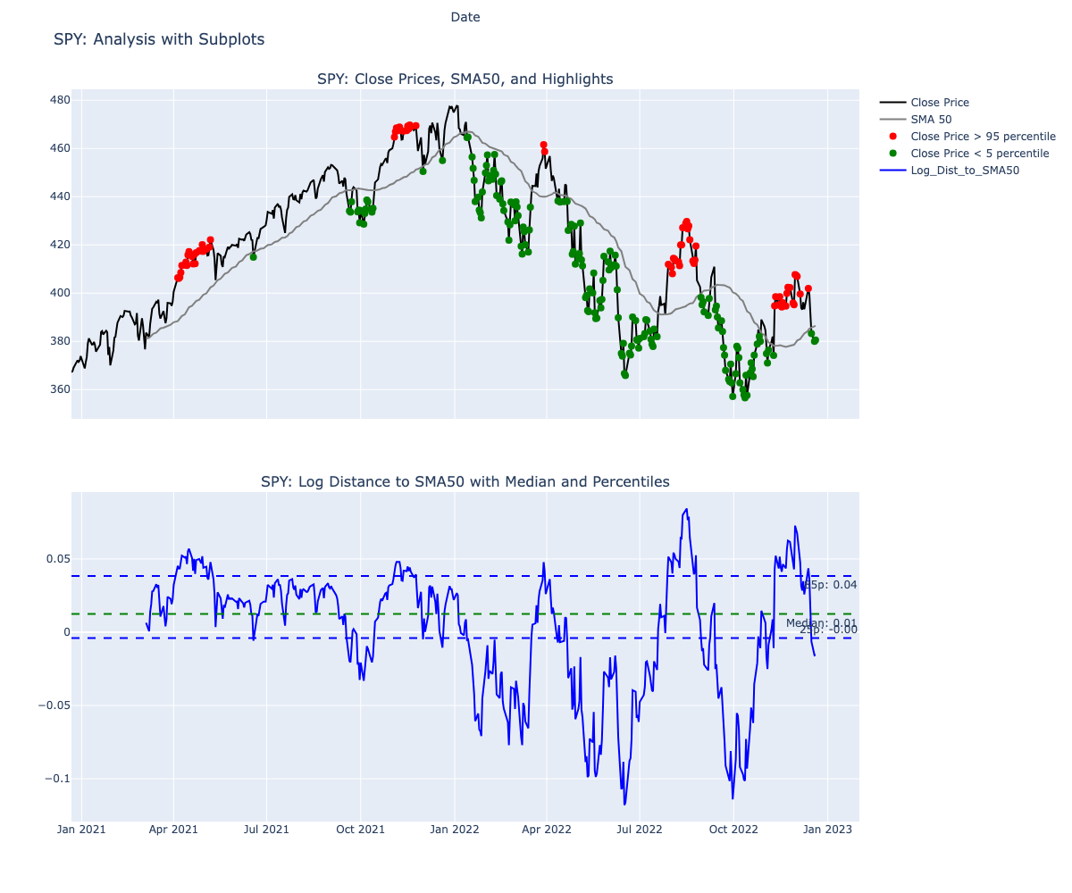
Simulating for SPY over 5 years again, this time with the bias fixes
We’ll use the validation dataset now : Here’s how the trades look for the validation dataset
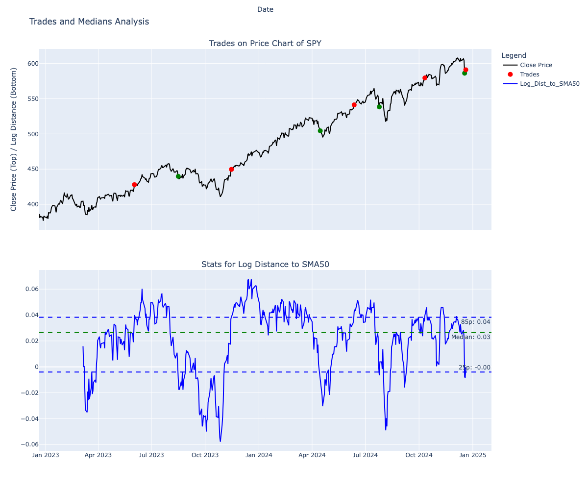
Sold 100 shares at: 427.92 on 2023-06-02 00:00:00
Profit/Loss for this trade: 4169.00
Bought 100 shares at: 439.64 on 2023-08-16 00:00:00
Sold 100 shares at: 449.68 on 2023-11-15 00:00:00
Profit/Loss for this trade: 1004.00
Bought 100 shares at: 504.45 on 2024-04-15 00:00:00
Sold 100 shares at: 541.36 on 2024-06-12 00:00:00
Profit/Loss for this trade: 3691.00
Bought 100 shares at: 538.41 on 2024-07-25 00:00:00
Sold 100 shares at: 579.58 on 2024-10-11 00:00:00
Profit/Loss for this trade: 4117.00
Bought 100 shares at: 586.28 on 2024-12-18 00:00:00
Sold remaining shares at: 591.15 on 2024-12-20 00:00:00
Profit for this trade: 487.00

Total Profit over 728 days: 13468.00
Buy and hold total profit: $20,492.00
Strategy Outcome: $-7,024.00
Which is a marked improvement from our -$18041.99 strategy deficit earlier - but still negative.
In summary: This seems slightly better on the extremes - but momentum is still making us buy on continued downward pressure, and also making us sell sooner, making the overall strategy loss making.
Fixing for momentum
A proper solution would be to factor the momentum into the equation when making our buy and sell decisions.
But that gets complex, by adding another variable to the mix - so i’ll delve into it in the future.
For now, let’s see if we can use options to fix the problem instead
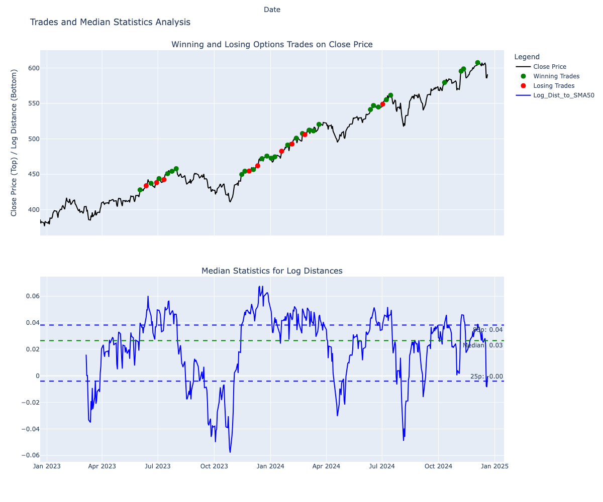
Key logic: We don’t want to have the opportunity loss of missing out on a strong bull run. But in cases when this indicator is right - it should generate us some extra cash. So let’s try to use a covered call to capitalise on the extremes. When the strategy is losing, we buy back our shares on the expiry date - and count the difference of prices as an opportunity loss.
Simulating a 1% premiums Covered-call option strategy
# Utility fn to find the next Friday
def get_next_friday(date):
    date = pd.to_datetime(date)
    # Get the weekday (Monday=0, ..., Sunday=6)
    weekday = date.weekday()
    # Calculate days to next Friday (weekday 4)
    days_to_friday = (4 - weekday + 7) % 7
    # If already Friday, move to the next Friday
    if days_to_friday == 0:
        days_to_friday = 7
    # Add the offset to the original date
    next_friday = date + pd.Timedelta(days=days_to_friday)
    return next_friday

def simulate_options(data, highlight_indices, highlight_low_indices):
  premium_percentage = 0.01  # 1% premium
  premiums_collected = 0  # Initialize total premiums collected
  opportunity_loss = 0  # Track opportunity loss when buying back shares
  strike_price_buffer = 0.01 # 1% above current price

  trade_log = []
  holding_option_until = pd.Timestamp.min  # Track until when we are holding an option

  for idx in highlight_indices:
      # Skip this index if we are already holding an option that hasn't expired
      if idx <= holding_option_until:
          continue

      # Current stock price at the sell signal
      stock_price = data.loc[idx, 'Close']
      # Premium collected from selling the option
      premium = stock_price * premium_percentage * 100
      # ATM strike price is the same as the current stock price
      strike_price = stock_price * (1 + strike_price_buffer)

      # Simulate option expiry
      holding_option_until = get_next_friday(idx)  # Get the price on the next Friday
      if holding_option_until not in data.index:
            continue
      next_friday_price = data['Close'][holding_option_until]

      if next_friday_price > strike_price:  # ITM
          # Calculate opportunity loss (difference between next Friday's price and strike price for 100 shares)
          # loss = premium * 1.5 # Bought back the option at 50% higher cost
          premiums_collected += premium
          loss = (next_friday_price - strike_price) * 100 # Got sold at strike price since
          opportunity_loss += loss
          # Log the transaction with the loss
          trade_log.append({
              'Index': idx,
              'Next Friday Date': holding_option_until,
              'Price': stock_price,
              'Strike Price': strike_price,
              'Next Friday Price': next_friday_price,
              'Outcome': 'ITM - Bought Back option',
              'Premium Collected': premium,
              'Opportunity Loss': loss
          })
      else:  # OTM
          # Add premium to total collected
          premiums_collected += premium
          # Log the transaction without loss
          trade_log.append({
              'Index': idx,
              'Next Friday Date': holding_option_until,
              'Price': stock_price,
              'Strike Price': strike_price,
              'Next Friday Price': next_friday_price,
              'Outcome': 'OTM - Premium Retained',
              'Premium Collected': premium,
              'Opportunity Loss': 0
          })

    # Convert log to DataFrame
  trade_log_df = pd.DataFrame(trade_log)

  return opportunity_loss, trade_log_df, premiums_collected
Results
Buy and Hold Strategy Base: 20492.00
-Opportunity Loss: 1312.18
Total profit excluding opp loss: 19179.82
+Total Premium: 17445.38
Strategy Delta: 16133.20
Wins: 28
Losses: 9
Win rate: 0.7567567567567568
So we made an additional ~$16,133!
This sounds great, but note that I’ve made a lot of assumptions here and this will likely fail when it goes to production against actual live data.
Here’s the graphical representation of all the trades. We (almost) never sell the stock, and we make more profitable covered call premiums than opportunity losses.
Conclusion
I think this simple strategy provides a lot of insights and learnings.
I made a ton of assumptions in the option simulations, that may not work with real datasets - but thats okay, the point is to learn for now and iterate.
Ignoring the momentum seems silly, let’s try to incorporate it next.
Congratulations for reading this far, I fix these issues and improve in Part 2: post